The Perfect Serve: What Tennis Taught Me About Reading PMM Like a Coach Instead of Guessing

When I started learning tennis as an adult, I realized that what made tennis difficult was not learning the tennis strokes, instead it was learning to realize the value of the feedback loop: racket vibrations, tennis ball sounds, and the way my balance shifted before I even realized it. None of this information is obvious on the court. However, without it I would continue to make the same significant error, and be frustrated that “trying harder” doesn’t seem to aid.

A similar realization came to me a few months ago, although this time was pretty different. Think of Percona Monitoring and Management (PMM) as the tennis racket and Percona Server for MySQL 8.0 as the tennis court. The measured result was a 95.0% reduction in average query time, from 54.17 ms to 2.71 ms. The only thing that changed was my perspective, not the setup.

The Setup

Very basic setup. One Percona Server for MySQL 8.0 primary, two EC2 read replicas, and PMM 2.x running in a Docker container, with QAN through performance_schema. Nothing special. The symptom was also standard: an internal analytics service joined three tables (orders, order_items, and users) and polled the primary every few minutes for recent order activity. None of the tables were big.

The screenshots and measurements in this walkthrough come from a lab environment created to reproduce the query pattern, not from a production incident.

In the baseline window, the query ran at 0.16 QPS and averaged 54.17 ms. It also lined up closely with CPU spikes and occasional replica-lag warnings.

My “power play” instinct kicked in, and I thought about increasing the resources for the primary, or moving the analytic workload totally over to a replica. Both ideas had potential, but at the end of the day, they would just hide the problem. None of the ideas actually would have helped me understand what the problem was.

Reading the Court: QAN Sorted by Load, Not Raw Query Time

The first real change in my mindset came from how I was sorting Query Analytics. The usual way to do this is to look for the query with the maximum or mean query time, and sort the results that way.

For this reason, PMM’s QAN dashboard has a Load column. Load is the average number of simultaneous executions of a query. Instead of looking at how long a query takes when executed, a better way to look at this is how much of the server’s attention is this query consuming, on average, right now. When sorting by Load, the three-table join jumped to the top. An average execution time of 54.17 ms does not look problematic until you realize the query is executed multiple times a minute, over and over again, continuously throughout the day.

That’s the first lesson: If a query never stops running, a query that is “fast enough” can still be your biggest rival.

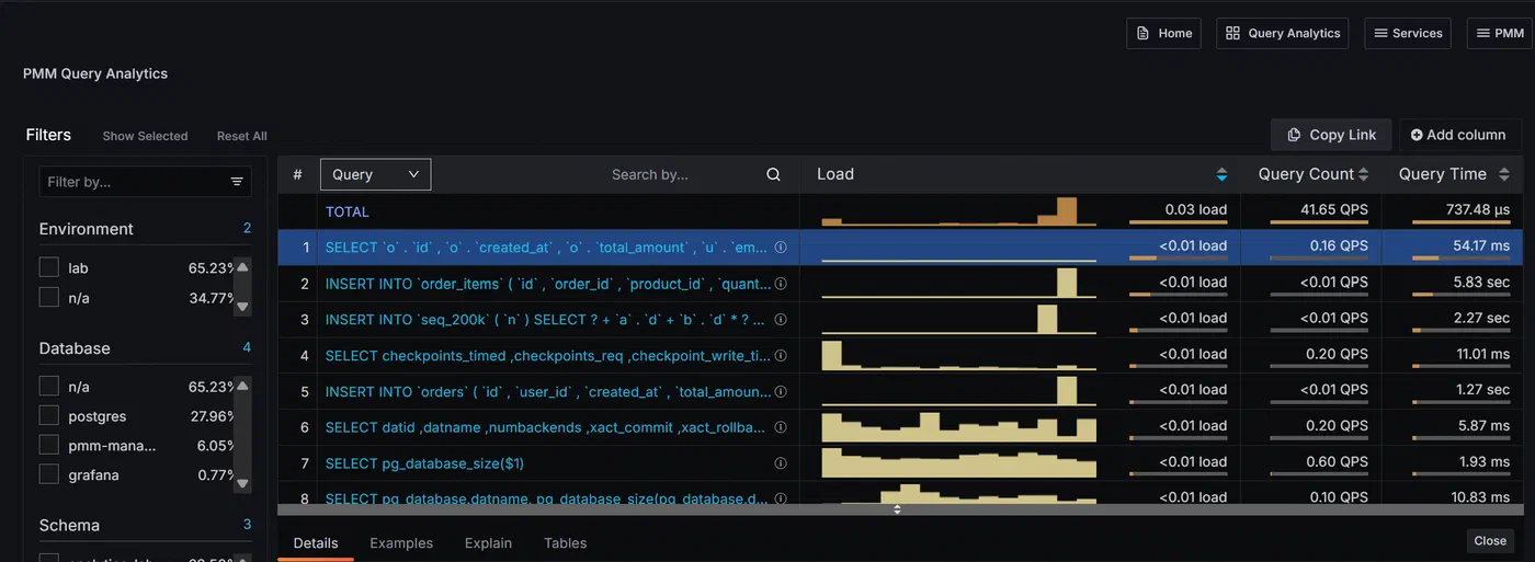
Figure 1: PMM Query Analytics showing the three-table join at the top of the workload, with an average query time of 54.17 ms before optimization.

Film Review Before Stepping on the Court: EXPLAIN

Once QAN pointed at the query, the next step was to observe EXPLAIN, as a coach would observe game film: review it before making any changes in production.

The query, in simplified form, looked like this:

SELECT o.id, o.created_at, o.total_amount, u.email,
oi.product_id, oi.quantity, oi.price
FROM orders o
JOIN order_items oi ON oi.order_id = o.id
JOIN users u ON u.id = o.user_id
WHERE o.created_at >= NOW() - INTERVAL 15 MINUTE
ORDER BY o.created_at DESC;

EXPLAIN confirmed this was a perfect example for a full table scan on orders (type: ALL). MySQL had to read every row to filter for the time window, then it used a nested loop to join order_items and users, which exacerbated the original issue.

orders:
type: ALL
key: NULL
rows: 199875
Extra: Using where; Using filesort
users:
type: eq_ref
key: PRIMARY
order_items:
type: ref
key: idx_order_items_order_id

Thanks to PMM’s rows examined to rows sent ratio, the query’s inefficiency actually showed itself where it could not in raw EXPLAIN output. The query would even return a reasonably sized and useful result. The issue was that the ratio of rows examined and rows sent to the client was totally lopsided. Each execution examined about 201,370 rows while returning 819 rows, or 245.87 rows examined for every row sent. This would not trigger any system alerts, but it showed that the database was doing SO much work for a trivial result. I’m calling this “invisible” inefficiency, and the more the query becomes used, the more detrimental it becomes.

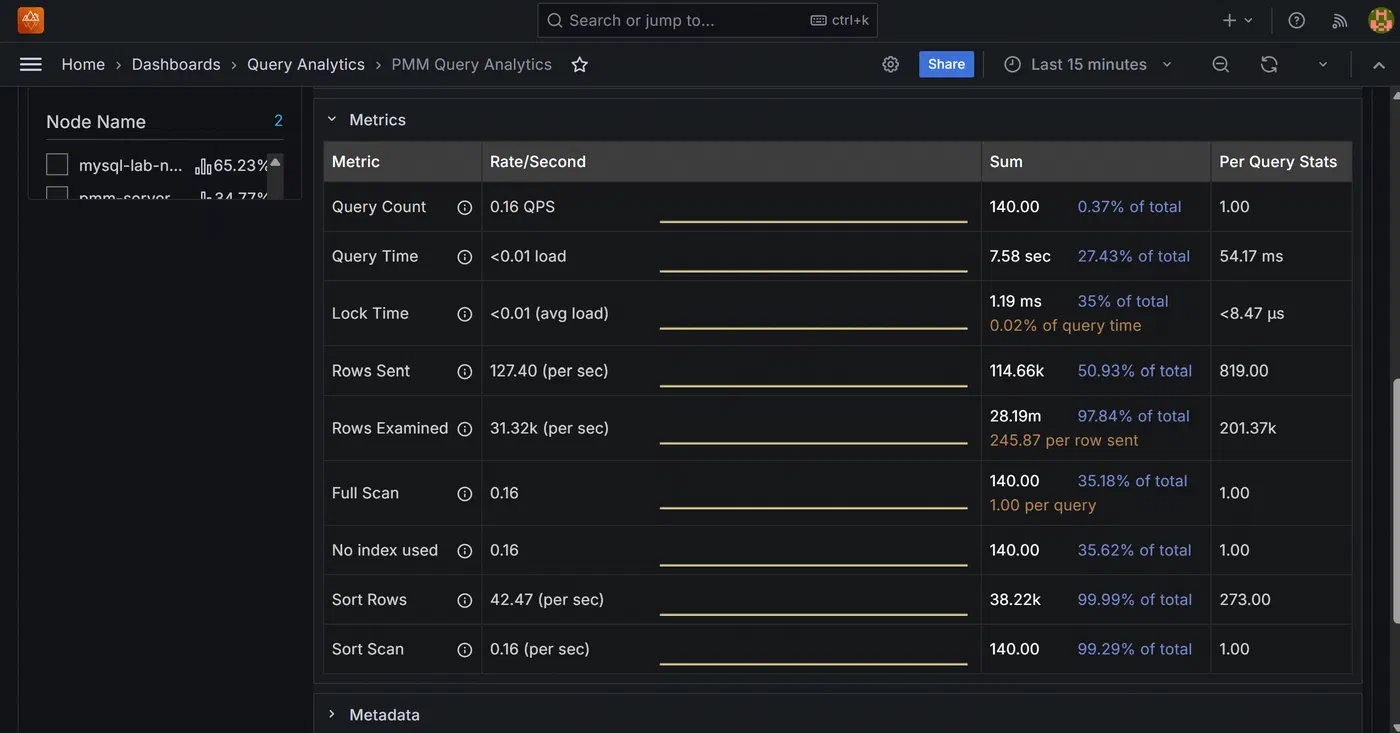
Figure 2: Before optimization, each execution examined about 201,370 rows while returning 819 rows, or 245.87 rows examined for every row sent. PMM also recorded a full scan and no index used on every execution.

The Fix: Small, Targeted Adjustments

This was actually the best example of tennis in the real world for me. The tendency in this sort of query optimization is to swing harder (a bigger instance, more read replicas, etc.), but this was more like lightly changing the grip by a few grams.

Two index changes, one query change, and that was it.

A composite index on orders that matches the access pattern:

CREATE INDEX idx_orders_created_at_id
ON orders (created_at, id);

The composite index on (created_at, id) allowed MySQL to use a range scan on the created_at predicate instead of scanning the entire orders table. In EXPLAIN, the orders access changed from type: ALL with roughly 199,875 rows estimated to type: range using idx_orders_created_at_id. The id column does not make this access covering, because the query still needs total_amount and user_id from the orders row.

A covering index on order_items:

CREATE INDEX idx_order_items_covering
ON order_items (order_id, product_id, quantity, price);

The covering index on (order_id, product_id, quantity, price) allowed MySQL to satisfy the join and requested item columns from the index itself. EXPLAIN reported Using index.

The last change was to split the users lookup from the main join. The first query returned user_id, and a second query used WHERE id IN (…) to fetch the email addresses from users.

None of these improvements required any downtime, schema redesigns, or having to talk about sizing the instances. Each improvement was the kind of adjustment where it looked like, on its own, nothing particularly important was actually done.

orders:
type: range
key: idx_orders_created_at_id
rows: 40
Extra: Using index condition; Backward index scan
users:
type: eq_ref
key: PRIMARY
order_items:
type: ref
key: idx_order_items_covering
Extra: Using index

The Results

The same normalized query remained at the top of the selected QAN workload after optimization, now running at 0.99 QPS and averaging 2.71 ms per execution.

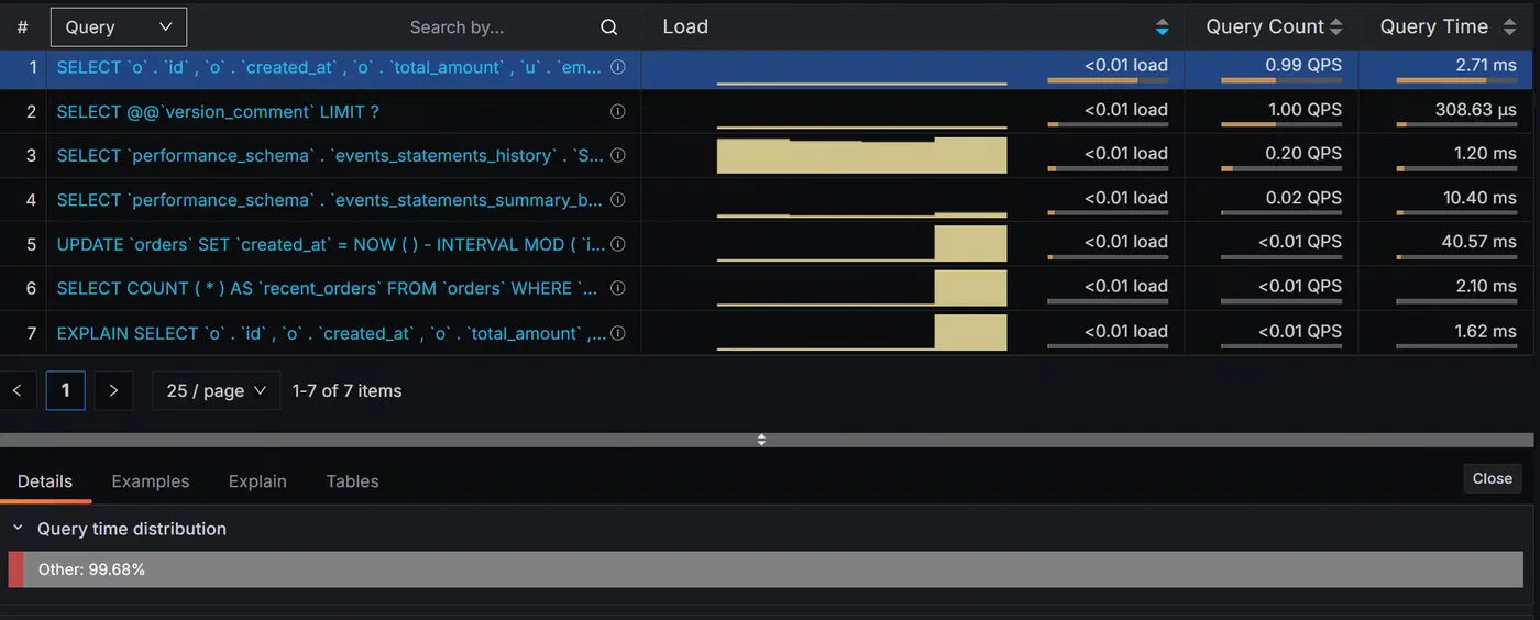
Figure 3: The same normalized query after optimization, now averaging 2.71 ms per execution in the post-index sampling window.

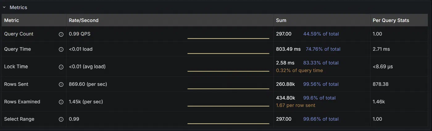
Figure 4: After the changes, average query time fell to 2.71 ms and rows examined dropped to about 1,460 per execution. The rows-examined-to-rows-sent ratio fell to 1.67, and executions used range access instead of a full scan.

Regarding the query, QAN indicated that average query time decreased from 54.17 ms to 2.71 ms, yielding a 95.0% reduction and making the query about 20 times faster. Rows examined per query fell from 201.37k to 1.46k, a 99.27% reduction, or about 138 times fewer rows examined. The ratio of rows examined to rows sent fell from 245.87 to 1.67, a 99.32% reduction. Full scan and no index used disappeared from the optimized sampling window, while Select Range reached 1.00 per query.

Improvements were the result of a number of incremental changes rather than a single large scale change. Composite indexing of orders and covering indexing of order_items helped rationalize the query to a considerable extent. Together, the changes rationalized the query and had an impact that would otherwise have been easy to chase with additional hardware.

Shifting Your Mindset

Beyond the specific indexes, the key point of this case study is how the investigation was framed at the outset.

QAN was sorted by Load. This let me identify the query that consumed the most attention from the primary. Unlike the query that had the most problematic single execution time.

Taking time to analyze EXPLAIN and the rows-examined-to-rows-sent ratio before implementing the fix let me focus on the cause of the problem. A full scan on orders. Instead of a symptom, which was a CPU spike with a concurrent lag on the replica.

By implementing two specific indexes and a small query rewrite, I ended up with measurable, attributable, and repeatable results. And if something was negatively impacted after the implementation of the fix, I would be able to identify which specific change caused the problem.

The engineer that looks as if they are moving the least in a tennis match, because they have already anticipated the next three shots, is the one doing the most invisible work, and that is exactly what this kind of production database work looks like from the outside.

PMM didn’t perform the optimization, but it made the invisible work just visible enough to act on the changes, and the rest was patience, and a willingness to implement incremental changes rather than larger changes.

About the author

Shivank Pandey is one of two engineers managing PMM at his company. He works with Percona Server for MySQL 8.0 in a primary-replica setup on EC2 and writes about database observability and query optimization.

This post is part of the Percona Community Writers Program. ∎